A Hero’s Journey to Deep Learning CodeBase Series – Part IIA
By Gal Hyams and Dan Malowany

Deep neural networks for object detection tasks is a mature research field. That said, making the correct tradeoff between speed and accuracy when building a given model for a target use-case is an ongoing decision that teams need to address with every new implementation. Although many object detection models have been researched over the years, the single-shot approach is considered to be in the sweet spot of the speed vs. accuracy trade-off. In this post (part IIA), we explain the key differences between the single-shot (SSD) and two-shot approach. Since its release, many improvements have been constructed on the original SSD. However, we have focused on the original SSD meta-architecture for clarity and simplicity. In the following post (part IIB), we will show you how to harness pre-trained Torchvision feature-extractor networks to build your own SSD model.
Why do we need this SSD model anyhow?
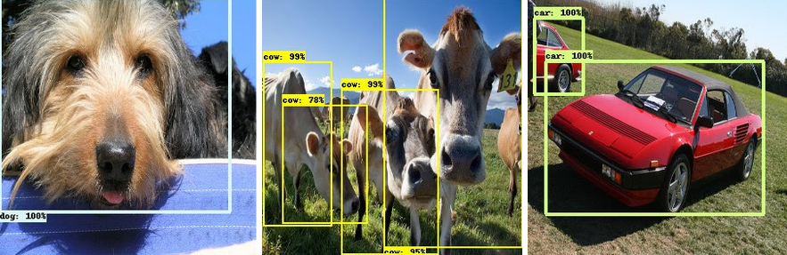
In object detection tasks, the model aims to sketch tight bounding boxes around desired classes in the image, alongside each object labeling. See Figure 1 below.
There are two common meta-approaches to capture objects: two-shot and single-shot detection.
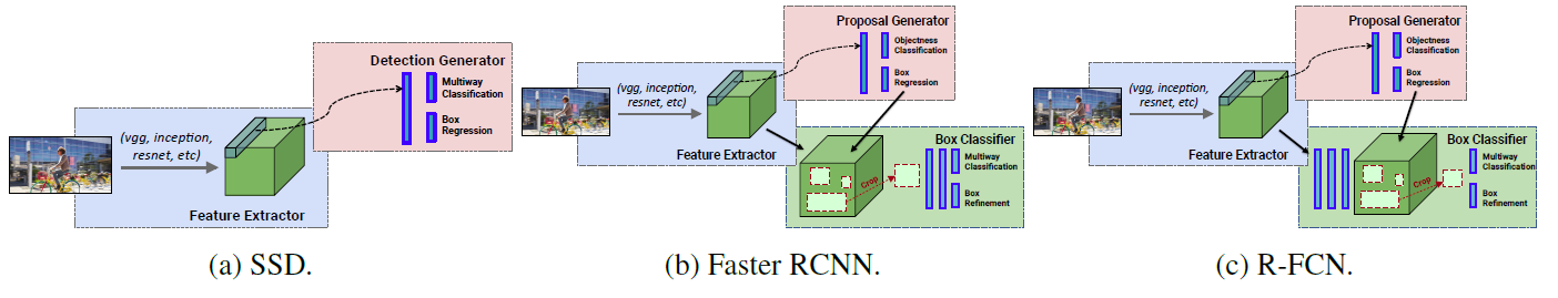
The two-shot detection model has two stages: region proposal and then classification of those regions and refinement of the location prediction. Single-shot detection skips the region proposal stage and yields final localization and content prediction at once. Faster-RCNN variants are the popular choice of usage for two-shot models, while single-shot multibox detector (SSD) and YOLO are the popular single-shot approach. YOLO architecture, though faster than SSD, is less accurate.
R-FCN (Region-Based Fully Convolutional Networks) is another popular two-shot meta-architecture, inspired by Faster-RCNN. In this approach, a Region Proposal Network (RPN) proposes candidate RoIs (region of interest), which are then applied on score maps. All learnable layers are convolutional and computed on the entire image. There, almost all of the different proposed regions’ computation is shared. The per-RoI computational cost is negligible compared with Fast-RCNN. R-FCN is a sort of hybrid between the single-shot and two-shot approach. When you really look into it, you see that it actually is a two-shot approach with some of the single-shot advantages and disadvantages.
While two-shot detection models achieve better performance, single-shot detection is in the sweet spot of performance and speed/resources. In addition, SSD trains faster and has swifter inference than a two-shot detector. The faster training allows the researcher to efficiently prototype & experiment without consuming considerable expenses for cloud computing. More importantly, the fast inference property is typically a requirement when it comes to real-time applications. As it involves less computation, it therefore consumes much less energy per prediction. This time and energy efficiency opens new doors for a wide range of usages, especially on end-devices and positions SSD as the preferred object detection approach for many usages.
Lately, hierarchical deconvolution approaches, such as deconvolutional-SSD (DSSD) and feature pyramid network (FPN), have become a necessity for any object detection architecture. The hierarchical deconvolution suffix on top of the original architecture enables the model to reach superior generalization performance across different object sizes which significantly improves small object detection. As our aim here is to detail the differences between one and two-shot detectors and how to easily build your own SSD, we decided to use the classic SSD and FasterRCNN.
Comparison between single-shot object detection and two-shot object detection
Faster-RCNN:
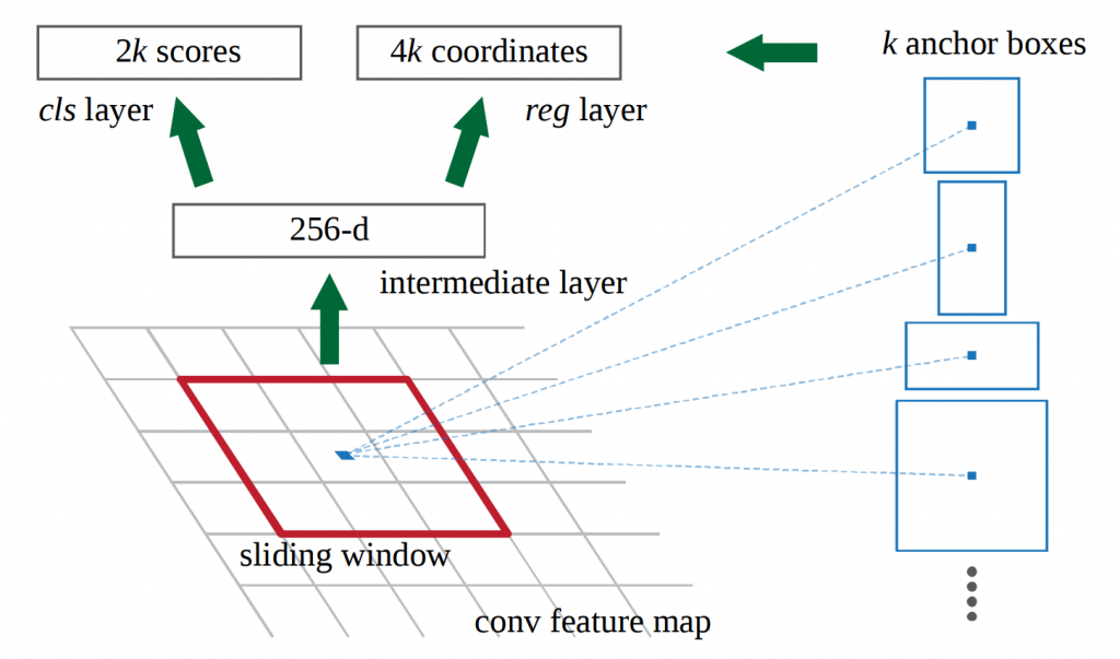
Faster R-CNN detection happens in two stages. The first stage is called region proposal. Images are processed by a feature extractor, such as ResNet50, up to a selected intermediate network layer. Then, a small fully connected network slides over the feature layer to predict class-agnostic box proposals, with respect to a grid of anchors tiled in space, scale and aspect ratio (figure 3).
In the second stage, these box proposals are used to crop features from the intermediate feature map which was already computed in the first stage. The proposed boxes are fed to the remainder of the feature extractor adorned with prediction and regression heads, where class and class-specific box refinement are calculated for each proposal.
Although Faster-RCNN avoids duplicate computation by sharing the feature-map computation between the proposal stage and the classification stage, there is a computation that must be run once per region. Thus, Faster-RCNN running time depends on the number of regions proposed by the RPN.
SSD:
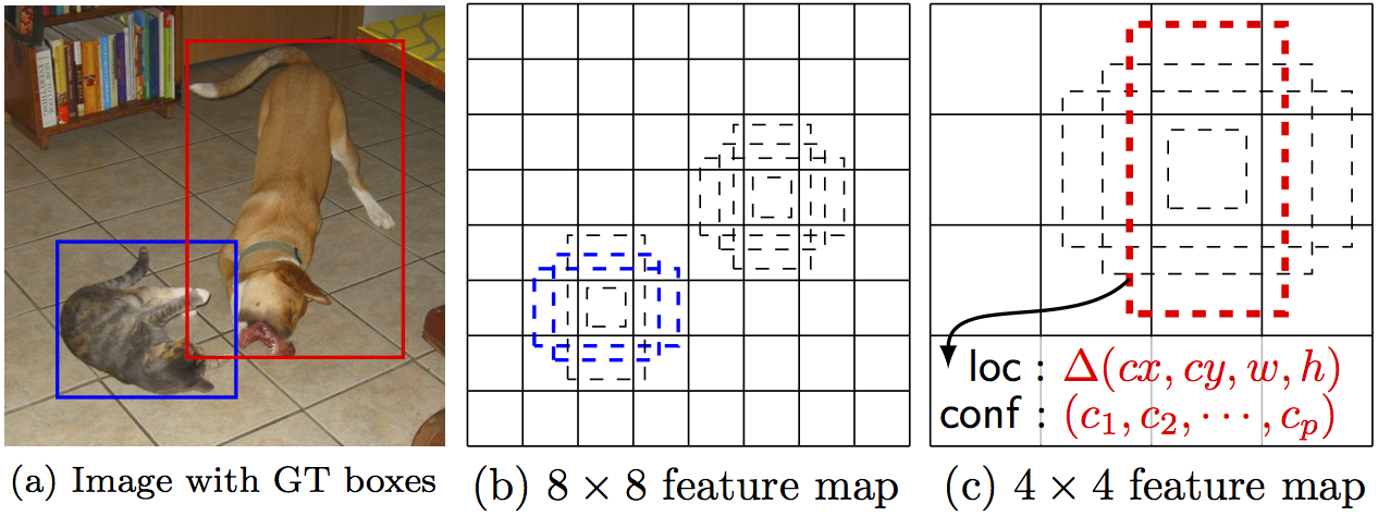
The SSD meta-architecture computes the localization in a single, consecutive network pass. Similar to Fast-RCNN, the SSD algorithm sets a grid of anchors upon the image, tiled in space, scale, and aspect ratio boxes (figure 4). As opposed to two-shot methods, the model yields a vector of predictions for each of the boxes in a consecutive network pass. This vector holds both a per-class confidence-score, localization offset, and resizing.
The class confidence score indicates the presence of each class instance in this box, while the offset and resizing state the transformation that this box should undergo in order to best catch the object it allegedly covers. To get a decent detection performance across different object sizes, the predictions are computed across several feature maps’ resolutions. Each feature map is extracted from the higher resolution predecessor’s feature map, as illustrated in figure 5 below.
The multi-scale computation lets SSD detect objects in a higher resolution feature map compared to FasterRCNN. FasterRCNN detects over a single feature map and is sensitive to the trade-off between feature-map resolution and feature maturity. SSD can enjoy both worlds. On a 512×512 image size, the FasterRCNN detection is typically performed over a 32×32 pixel feature map (conv5_3) while SSD prediction starts from a 64×64 one (conv4_3) and continues on 32×32, 16×16 all the way to 1×1 to a total of 7 feature maps (when using the VGG-16 feature extractor).
The separated classifiers for each feature map lead to an unfortunate SSD tendency of missing small objects. Usually, the model does not see enough small instances of each class during training. Zoom augmentation, which shrinks or enlarges the training images, helps with this generalization problem. On the other hand, SSD tends to predict large objects more accurately than FasterRCNN. Figure 4 illustrates the anchor predictions across different feature maps. Why SSD is Faster than Faster-RCNN?
Why SSD is Faster than Faster-RCNN?
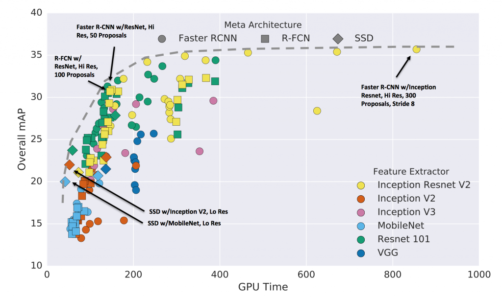
As can be seen in figure 6 below, the single-shot architecture is faster than the two-shot architecture with comparable accuracy. There are two reasons why the single-shot approach achieves its superior efficiency:
- The region proposal network and the classification & localization computation are fully integrated. This minimizes redundant computations.
- Single-shot is robust with any amount of objects in the image and its computation load is based only on the number of anchors. However, Faster-RCNN computations are performed repetitively per region, causing the computational load to increase with the number of regions proposed by the RPN. This number is limited by a hyper-parameter, which in order to perform well, is set high enough to cause significant overhead. R-FCN only partially minimizes this computational load. On top of the SSD’s inherent talent to avoid redundant computations, figure 6 shows this meta-architecture successfully harnessing efficient feature extractors, such as MobileNet, and significantly outperforms two-shot architectures when it comes to being fed from these kinds of fast models.
Why SSD is less accurate than Faster-RCNN?
The Focal Loss paper investigates the reason for the inferior single-shot performances. After all, it is hard to put a finger on why two-shot methods effortlessly hold the “state-of-the-art throne”. The paper suggests that the difference lies in foreground/background imbalance during training.
Two-stage detectors easily handle this imbalance. The RPN narrows down the number of candidate object-locations, filtering out most background instances. On top of this, sampling heuristics, such as online hard example mining, feeds the second-stage detector of the two-stage model with balanced foreground/background samples. In contrast, the detection layer of a one-stage model is exposed to a much larger set of candidate object-locations, most of which are background instances that densely cover spatial positions, scales, and aspect ratios during training. While two-shot classifier sample heuristics may also be applied, they are inefficient for a single-shot model training as the training procedure is still dominated by easily classified background examples. The Focal Loss approach concentrates the training loss on difficult instances, which tend to be foreground examples. In doing so, it works to balance the unbalanced background/foreground ratio and leads the single-shot detector into the hall of fame of object detection model accuracy.
So what’s the verdict: single-shot or two-shot?
It’s clear that single-shot detectors, with SSD as their representative, are more cost-effective compared to the two-shot detectors. They achieve better performance in a limited resources use case. Moreover, when both meta-architectures harness a fast lightweight feature-extractor, SSD outperforms the two-shot models. On the other hand, when computing resources are less of an issue, two-shot detectors fully leverage the heavy feature extractors and provide more reliable results. The main hypothesis regarding this issue is that the difference in accuracy lies in foreground/background imbalance during training. Leveraging techniques such as focal loss can help handle this imbalance and lead the single-shot detector to be your choice of meta-architecture even from an accuracy point of view.
The next post, part IIB, is a tutorial-code where we put to use the knowledge gained here and demonstrate how to implement SSD meta-architecture on top of a Torchvision model in Allegro Trains, our open-source experiment & autoML manager.
Be in touch with any questions or feedback you may have!