The design and training of neural networks are still challenging and unpredictable procedures. The difficulty of tuning these models makes training and reproducing more of an art than a science, based on the researcher’s knowledge and experience. One of the reasons for this difficulty is that the training procedure of machine learning models includes multiple hyperparameters that affect how the training process fits the model to the data. These hyperparameters directly control the behaviors of training algorithms and have a significant effect on the performance of the resulting machine learning models. Unlike the internal model parameters, such as the neural network’s weights, which can be learned from the data during the model training phase, hyperparameters are set prior to the learning process.
he most widely used method for hyperparameter optimization is the manual tuning of these hyperparameters, which demands professional knowledge and expert experience. However, in many cases, past experience in training neural networks is not enough and researchers resort to a brute-force grid search. In addition, relying on past experience generally provides workable, instead of an optimal, hyper-parameter set. To lower the technical thresholds for common users, automated hyper-parameter optimization has become a popular topic in recent years.
his blog post is a second of a series on how to leverage PyTorch’s ecosystem tools to easily jumpstart your ML/DL project. This blog post focused on introducing ClearML, the new member of the PyTorch ecosystem, and demonstrating how it enables reproducibility, improves teamwork, easy experiment management and efficient MLOps. In this blog post, we will show how using ClearML’ built-in integration with Optuna, another PyTorch Ecosystem project, enables simple, accurate and fast hyperparameter optimization.
The Hyperparameter Optimization Challenge
Traditionally, hyperparameter optimization has been the job of humans because they can be very efficient in regimes where only a few trials are possible. This manual optimization method, which is sometimes called “the graduate student search” or simply “babysitting”, is considered computationally efficient if you have a team of researchers with vast experience using the same model on highly similar data. Even then, it is plausible mainly in cases where the number of hyperparameters to tune is small. However, it naturally relies on highly trained manual labor and reaches workable but not optimal results. Furthermore, this is a serial process, as this is a trial and error process where the researcher needs to learn from previous trials and tune the parameters of the following trials. In a world where computer clusters and GPU processors make it possible to run abundant trials in parallel, the man in the loop may become the bottleneck of the optimization process. As a result, the field of automated hyper-parameter optimization started to gain interest in the machine learning community. Before we cover some of the most popular and efficient automatic optimization techniques, it is important to note that having a human in the loop gives researchers some degree of insight into the hyperparameter function we aim to optimize. Such insight is essential to the researcher’s ability to improve the model and training algorithm continuously. Therefore the human man in the loop should be. kept to some degree in any automated process and make sure that the optimization process is visible to the data scientist.
Several automatic optimization methods gained popularity in recent years. The most popular ones being:
- Grid search — In grid search we choose a set of values for each parameter and the set of trials is formed by assembling every possible combination of values. It is simple to implement and trivial to parallelize. However, it suffers from the curse of dimensionality because the number of joint values grows exponentially with the number of hyper-parameters.
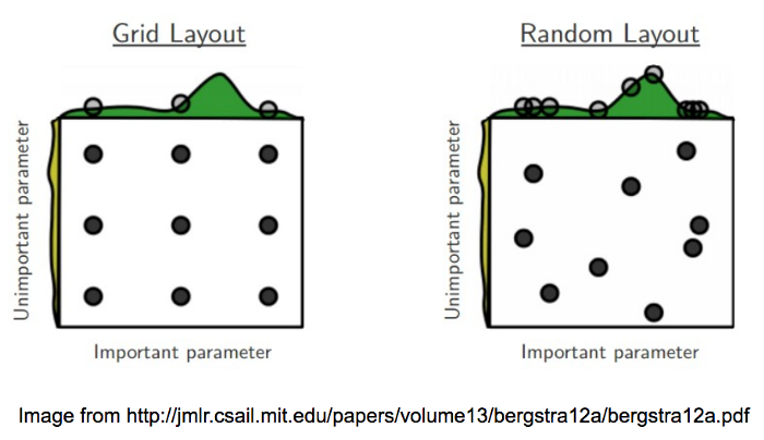
- Random search — Random search is considered a variation of grid search, where you independently draw random values from a uniform density from the same configuration space as would be spanned by a grid search. Random search has all the practical advantages of grid search (simplicity, ease of implementation, trivial parallelism) and trades a small reduction in efficiency in low-dimensional spaces for a large improvement in efficiency in high-dimensional search spaces. It is more efficient than grid search in high-dimensional spaces because the hyper parameter function we aim to optimize is more sensitive to changes in some dimensions than others. This makes random search the baseline against which more advanced hyper-parameter optimization algorithms are compared to. The superiority of random search over grid search due to the fact that some hyperparameters are more important than others is demonstrated in the next figure:
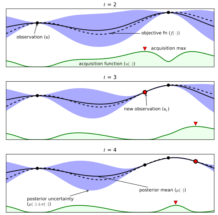
- Bayesian optimization — Bayesian optimization framework has several key ingredients. The main ingredient is a probabilistic surrogate model, which consists of a prior distribution that captures our beliefs about the behavior of the unknown objective function. It also includes an observation model that describes the data generation mechanism. After observing the output of each query of the objective, the prior is updated to produce a more informative posterior distribution over the space of objective functions. For better efficiency, Bayesian optimization uses acquisition functions to trade off exploration and exploitation; their optima are located where the uncertainty in the surrogate model is large (exploration) and/or where the model prediction is high (exploitation). Bayesian optimization algorithms then select the next query point by maximizing such acquisition functions as can be seen in the next figure. Although Bayesian optimization performs better than grid search and random search, in its naive form it has two main drawbacks: it is not a parallel algorithm and it works only on continuous hyper-parameters and not categorical ones. For both these issues, several variations of Bayesian optimization have been developed in recent years.
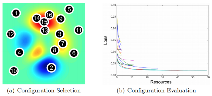
- Hyperband optimization — While Bayesian optimization aims to be more efficient and faster than standard baselines, like random search, by selecting hyper-parameters configuration in an adaptive manner, it needs to tackle the fundamentally challenging problem of simultaneously fitting and optimizing a high-dimensional, non-convex function with unknown smoothness, and possibly noisy evaluations. Hyperband is a general-purpose technique that avoids this problem by making minimal assumptions and focuses on addressing how to allocate resources among randomly sampled hyperparameter configurations. Hyperband is essentially a variation of random search that uses principled early-stopping strategy and an extension of the SuccessiveHalving algorithm to allocate resources. As a result, Hyperband evaluates more hyperparameter configurations and is shown to converge faster than Bayesian optimization on a variety of deep-learning problems, given a defined resources budget. A demonstration of how configuration evaluation methods, such as Hyperband, allocate more resources to promising configurations using early stopping, can be seen in the next figure:
Automatic optimization techniques keep evolving all the time with newer and improved algorithms being published every couple of months. We encourage the reader to explore these newer algorithms, such as BOHB (Bayesian Optimization and HyperBand) that mixes the Hyperband algorithm and Bayesian optimization, and PBT (Population-Based Training) which mixes ideas from genetic optimization algorithms, and others.
Using PyTorch Ecosystem to Automate your Hyperparameter Search.
PyTorch’s ecosystem includes a variety of open source tools that aim to manage, accelerate and support ML/DL projects. In this blog we will use two of these tools:
- ClearML is an open-source machine learning and deep learning experiment manager and ML-Ops solution. It boosts the effectiveness and productivity of AI teams as well as on-prem and cloud GPU utilization. The powerful and scalable design of ClearML helps researchers and developers to manage complex machine learning projects with zero integration effort.
- Optuna is an open source automatic hyperparameter optimization framework, particularly designed for machine learning. Thanks to its modular design and use of modern optimization functionalities, it enjoys a lightweight architecture that supports parallel distributed optimization and pruning of unpromising trials.
ClearML integrated Optuna’s functionality into their hyper parameter optimization module. Therefore, if you already use ClearML you can easily enjoy Optuna’s great functionality, while ClearML’ MLOps will take care of the optimization parallelism on your machines. In addition, ClearML’ experiment management will make sure your researchers will have full visibility into the optimization process, which will enable them to continue improving their model and code base.
To demonstrate the ease of use of these two packages in combination, we will continue the simple image processing example. The full code can be found here.
Hyperparameter Optimization with ClearML and Optuna
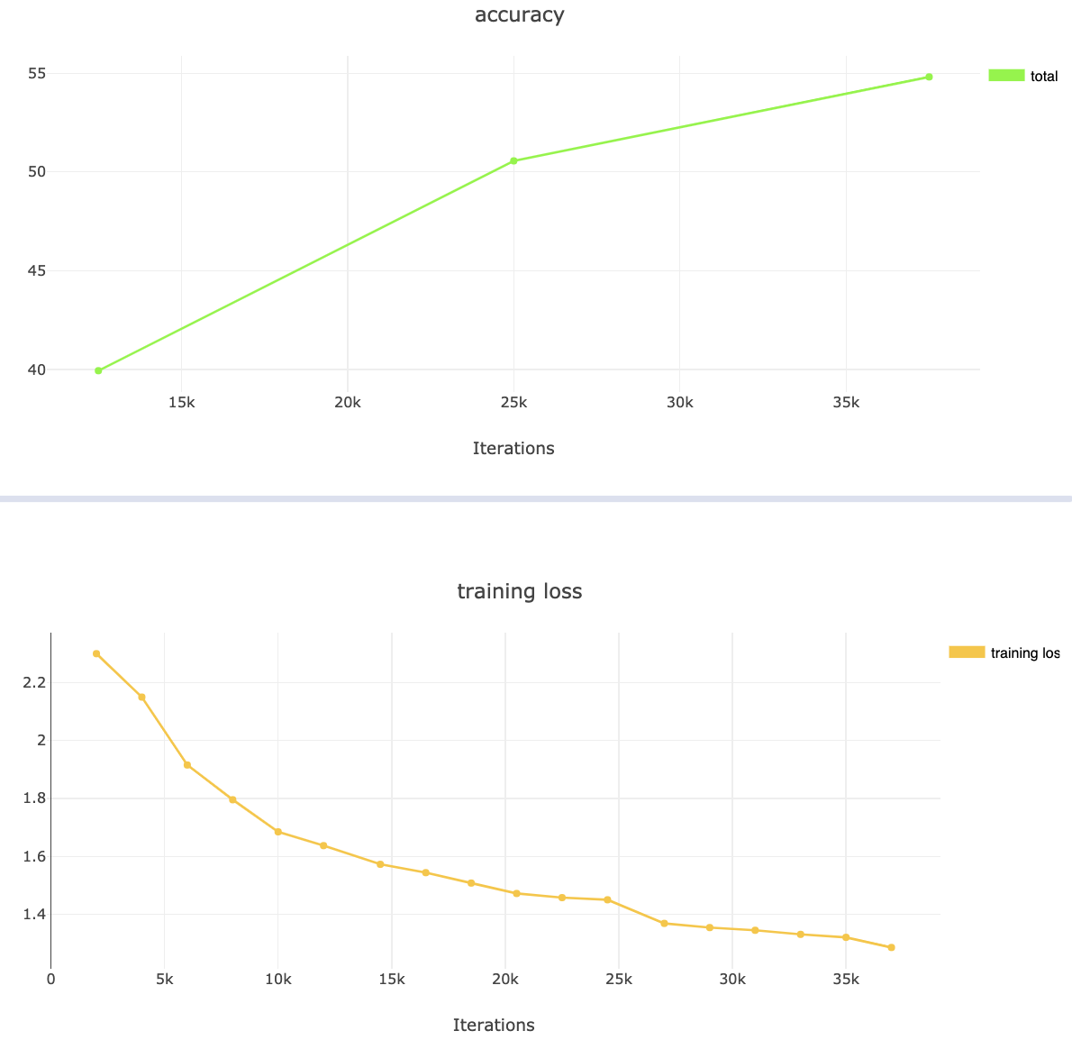
For simplification, we will not explain in this blog how to install a ClearML-server. Therefore, the experiment will be logged on the ClearML demo server. If you are using a self-hosted ClearML-server, you will start by executing the Pytorch image classification script from the previous blog. Otherwise, you can just use the already executed experiment in the demo server, which can be found here. Once executed, you can watch its progress in the ClearML’ webapp. ClearML not only logs all your accuracy and loss reports, but also adds status reports on the machine and its GPU.
Now that we verified there are no bugs and the experiment was logged successfully as well as converged as expected, it is time to initiate the hyperparameter optimization process. It is worth noting that we separate the training script from the optimization script, as the optimization script is general and can be used on numerous training scripts, no matter what is the model (SSD, Faster RCNN, etc) or even the task type (object detection, semantic segmentation, etc).
We will start by importing ClearML’ automation modules:
The HyperParameterOptimizer class contains ClearML’ hyperparameter optimization modules. Its modular design enables using different optimizers, such as Optuna, hpbandster’s BOHB and more. Optuna is the default optimizer in ClearML, so no need to import it. Nevertheless, in order to demonstrate the HyperParameterOptimizer syntax, we included it in this example.
Next we will add ClearML’ two lines of integration:
Now we will define the optimization configuration and resources budget. The main parameter to define are:
- base_task_id
This is the experiment we want to optimize. We can choose any experiment in ClearML’ webapp and copy the experiment ID. If you are using the demo app, you just click the ID symbol here. - hyper_parameters
These are the hyperparameters we want to optimize. Each experiment has its hyperparameters reflected in the experiment manager web app. If you use the well known argparse package, ClearML will automatically pick them up. Or you can just define them manually, as explained in our previous blog). Here you just define which of them to optimize and what are the values’ types and ranges. If you are using the demo app, you can find the list of hyperparameters of our experiment here. - objective_metric_title
This is the objective metric we want to optimize — It is simply the title of the scalars plot in the webapp, where the metric is logged. If you are using the demo app, you can find it here. - objective_metric_series
This is the objective metric we want to optimize — It is simply the series name of the scalar. If you are using the demo app, you can find it here. - objective_metric_sign
This defines whether to maximize or minimize the objective metric. - max_number_of_concurrent_tasks
This defines the maximum number of concurrent experiments to spawn, which limits the number of
workers the optimization process can occupy in parallel. - optimizer_class
This is the optimization class to use. By default it is set to be OptimizerOptuna. It can be changed to any of the following: GridSearch, RandomSearch or OptimizerBOHB. Make sure to import the class from clearml.automation. - execution_queue
This is the name of the queue to use for the optimization process. - total_max_jobs
The maximum number of experiments for the entire optimization process. - max_iteration_per_job
The maximum number of iterations per experiment, until early stopping. - optimization_time_limit
The time limit for the duration of the optimization process. - compute_time_limit
The total compute time allowed for the optimization process (sum of execution time on all machines). This enables limiting the computation cost, if using cloud machines.
That’s it — we are ready to go.
Before we initiate the optimization process, we need to make sure we have workers listening to the queue we have defined above. Setting the workers is done using ClearML Agent, the ML-Ops component of ClearML that spins a container for you on a remote machine and runs your code. This is a very simple process that we have described in our previous blog post. It needs to be done on each machine designated for executing the experiments.
Now all we have got left is to start the hyperparameter optimization process:
Now sit back and watch ClearML and Optuna do the job for you. The optimization project will be filled with all the optimization experiments as well as a master experiment that accumulates the optimization process and its progress.
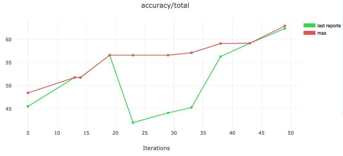
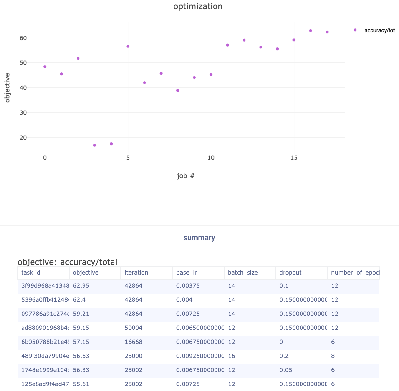
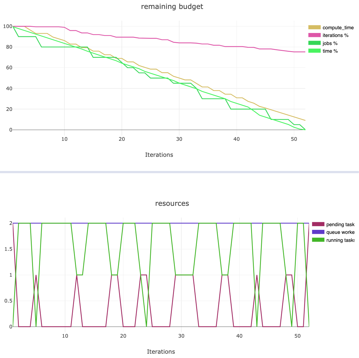
In addition to summarizing results from all experiments, the master experiment tracks the optimization budget (time, compute time, jobs, iteration) and resources (workers utilization).
Note that Optuna uses Tree-structured Parzen Estimator (TPE), which is a kind of Bayesian optimization, as the default sampler. It also uses Median pruner as the default pruner, although Optuna also supports Hyperband pruner, which performs better [source].
Summary
Hyperparameter search is one of the most cumbersome tasks in machine learning projects. It requires adjustments to the hyperparameters over the course of many training trials to arrive at the optimal values and the best performing model. The popular method of manual hyperparameter tuning makes the hyperparameter optimization process slow and tedious.
You can accelerate your machine learning project and boost your productivity, by leveraging the PyTorch ecosystem. This ecosystem of open source tools, includes tools for hyperparameter optimization, experiment management, MLOps and more.
In this tutorial we demonstrated ClearML’ built-in support for Optuna. With zero integration efforts and no cost, you get a simple and powerful method for an efficient and accurate hyperparameter optimization of your Pytorch training process, on top of ClearML’ experiment management system and ML-Ops solution.
To learn more reference to ClearML’ documentation and Optuna’s documentation. In the next blog post of this series we will demonstrate audio classification with Torchaudio and ClearML.